Next: GEM field equation solutions Up: Unifying gravity and electromagnetism Previous: Lagrange densities
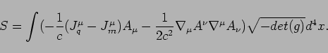
Write out the action based on the GEM Lagrange density (3):
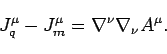
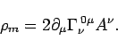
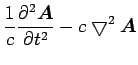
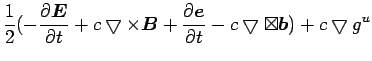
Varying the action by the 4-potential field generates the field equations:
This is a four-dimensional wave equation with two sources, one for
electricity, the other for gravity. The Maxwell equations are apparent
in the physical situation where the mass current density ![]() is effectively zero (all charged particles have a non-zero mass, but
the charge mass charge is more than thirteen orders of magnitude smaller
than the electric charge). The gauge is not fixed in the Lagrangian,
so there is more freedom, a necessity if the equation is also going
to describe gravity. Newton's field equation for gravity is the first
static field equation when there is no electric current density
is effectively zero (all charged particles have a non-zero mass, but
the charge mass charge is more than thirteen orders of magnitude smaller
than the electric charge). The gauge is not fixed in the Lagrangian,
so there is more freedom, a necessity if the equation is also going
to describe gravity. Newton's field equation for gravity is the first
static field equation when there is no electric current density ![]() .
The field equations are covariant under a Lorentz transformation,
behaving like a 4-vector. One of the justifications for general relativity
- to make Newton's field equation for gravity covariant under a Lorentz
transformation - is no longer compelling because 5
is manifestly covariant.[9]
.
The field equations are covariant under a Lorentz transformation,
behaving like a 4-vector. One of the justifications for general relativity
- to make Newton's field equation for gravity covariant under a Lorentz
transformation - is no longer compelling because 5
is manifestly covariant.[9]
Because the metric was not varied, that indicates that it must be fixed. With the Maxwell equations, there are no constraints on the metric, so a metric must be supplied as part of the background structure for the theory. For a connection that is metric compatible and torsion-free, second-order derivatives of the metric are part of the field equations. The process of finding solutions to the field equations will necessitate constraints on the dynamics of the metric. The rest of the background structure for the Maxwell equations - things like the 4-dimensional structure, the differential manifold - will still be necessary for the GEM field equations.
The classical fields can be expressed in terms of covariant derivatives
of the potential. The symmetric and antisymmetric field strength tensors
are very similar, differing only in the sign of the tensor
![]() .
The electric field
.
The electric field ![]() and magnetic field
and magnetic field ![]() together represent all the information in the antisymmetric field
strength tensor. Symmetric analogs
together represent all the information in the antisymmetric field
strength tensor. Symmetric analogs ![]() and
and ![]() are defined to do a similar job for the symmetric field strength tensor.
In addition, there is a four component field for the terms along the
diagonal which will be noted as
are defined to do a similar job for the symmetric field strength tensor.
In addition, there is a four component field for the terms along the
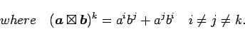
diagonal which will be noted as ![]() . To make a connection to
the classical fields of gravity and electromagnetism, use the following
mappings:
. To make a connection to
the classical fields of gravity and electromagnetism, use the following
mappings:
The set of five classical fields will transform like a second-rank asymmetric tensor. Under a Lorentz transformation, the three gravity fields will mix, as will the two electromagnetic fields. There will be no mixing between gravity and electromagnetic fields since the fields are in different, irreducible tensors.
The first row and column of the asymmetric field strength tensor is
the sum of the electric field ![]() and the symmetric analog
and the symmetric analog
![]() . The rest of the off-diagonal terms are the sum of the
magnetic field
. The rest of the off-diagonal terms are the sum of the
magnetic field ![]() and its symmetric counterpart
and its symmetric counterpart ![]() .
The diagonal of the field strength tensor is
.
The diagonal of the field strength tensor is ![]() . The sum of
the components of
. The sum of
the components of ![]() is the Lorentz invariant trace of the
asymmetric field strength tensor. The trace contains information about
both the electromagnetic gauge and the Christoffel symbols. The ability
to choose an arbitrary electromagnetic gauge is equivalent to ignoring
constraints imposed by gravity, which is common for all practical
problems with electromagnetism.
is the Lorentz invariant trace of the
asymmetric field strength tensor. The trace contains information about
both the electromagnetic gauge and the Christoffel symbols. The ability
to choose an arbitrary electromagnetic gauge is equivalent to ignoring
constraints imposed by gravity, which is common for all practical
problems with electromagnetism.
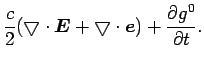
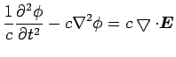
Substitute the classical fields (6-10) into the field equations (5), starting with the first field equation:
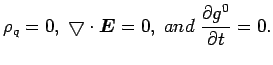
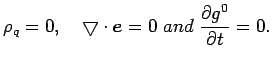
This has Gauss' law and analogous equation for gravity. One must note that the divergence with a contravariant derivative introduces another minus sign. The Newtonian gravitational field equation is embedded here under the following physical conditions:
If the time derivative of ![]() is not zero, then the field equations
for gravity incorporate time directly. This is significant because
one justification for general relativity is to make the form of Newton's
field equations dynamic.[11, chapter 7]
is not zero, then the field equations
for gravity incorporate time directly. This is significant because
one justification for general relativity is to make the form of Newton's
field equations dynamic.[11, chapter 7]
With a particular choice of reference frame such that all symmetric derivatives of the potential vanish, the relativistic form of 12 concerns changes in the Christoffel symbol exclusively:
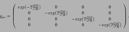
The second-order change in the metric is determined by the mass charge density. It is significant that the Riemann curvature tensor is not being used here because this unification model is fundamentally distinct from general relativity. One can find a metric which solves 13. For a static, non-rotating, uncharged mass where the change in the potential is zero, the exponential metric is a solution:
As the exponent goes to zero, the metric becomes the Minkowski metric for flat spacetime in the limit. The exponential metric equation has been studied previously.[12,17,6,15] The metric is consistent with weak field tests of gravity to first-order parameterized post-Newtonian (PPN) accuracy. At second-order PPN accuracy, light will bend around the Sun an additional 11.5 microarcseconds more than first order. General relativity predicts a second-order contribution of 10.8 microarcseconds.[2] At the current time, we can only measure light bending to 100 microarcseconds, and there are no experiments planned to determine the second-order PPN coefficients (Clifford Will, personal communication). In the future, the 0.7 microarcseconds difference in light bending represents a means to either confirm or reject this proposal.
Strong gravitational field tests such as the energy loss by binary pulsars due to gravity waves has ruled out Rosen's bimetric proposal. There can be a dipole mode of gravity wave emission due to the additional metric field. For the GEM model, there is no additional field to store energy or momentum, so for an isolated source, the lowest mode of emission is a quadrapole, consistent with the data from pulsars.
Gauss' law can be isolated under different physical conditions:
 |
(15) | ||
 |
To make the discussion of unification more concrete, imagine a proton
at the center of a 1 cm sphere. The electric charge density would
be
![]() . The mass charge density would be
. The mass charge density would be
![]() , thirteen orders of magnitude smaller
than the electric charge density. This model does not address why
there is such a significant difference between the charges. The unified
charge density for a proton is slightly less than the electric charge
density, although not measurably so since the electric charge is not
known to thirteen significant digits.
, thirteen orders of magnitude smaller
than the electric charge density. This model does not address why
there is such a significant difference between the charges. The unified
charge density for a proton is slightly less than the electric charge
density, although not measurably so since the electric charge is not
known to thirteen significant digits.
Repeat the exercise for the 3-vector field equation.
 |
(16) | ||
 |
This has Ampere's law and a symmetric analog for gravity.
The model for classical gravitational and electromagnetic field equations is expressed with 4-vectors, tensors of rank one. Einstein's field equations use tensors of rank two. Therefore the two approaches are fundamentally different. Although the field equations are rank one, the field strength tensor is second rank, consistent with arguments that a symmetric second-rank field strength tensor is required to characterize a dynamic metric. Second-order derivatives of the metric arise from the divergence of the Christoffel symbols as seen in 13.
The homogeneous Maxwell equations are vector identities, unaffected by unification.